|
|
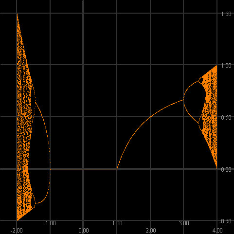
Usually the logistic function fc(x) = cx(1-x) is used to model population changes, and so the parameter c is taken positive. But if we allow for negative c values, we get two "copies" of the usual orbit diagram. The "copy" on the right is the "usual one" seen in illustrations. This image was created by iterating the critical number 1/2. |
|
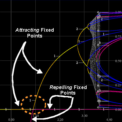
Here's a superimposition of the bifurcation diagram (through period 4) on the
"right side" of the orbit diagram. Periodic
points are colored according to the slope of fcn.
Attracting periodic points are colored yellow (slopes from -1 to 0) or orange (0 to +1) in the image.
A repelling periodic point is colored blue if the slope of
fcn(p) is less than -1 and fuschia if it's greater than +1.
An interesting feature of the logistic function is that it sports a transcritical bifurcation at c=1, marked inside the orange oval. There are two intersecting curves of fixed points. At c=1, they "exchange" their attracting/repelling natures. Curves on the bifurcation diagram are colored by prime period and automatically labeled by my program. |
|
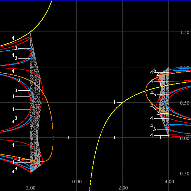
Here's a superimposition of the bifurcation diagram (through period 4)
on "both sides" of the orbit diagram. Curves on the bifurcation diagram are colored by prime period and automatically labeled by my program.
Compare the bifurcation diagrams for fc(x) = x2 + c and the logistic function shown here: The former's two curves of fixed points are "born" through the standard saddle node bifurcation at c=0.25. But here, one curve of fixed points is simply the horizontal line x=0. The other "breaks" at c=0: The vertical axis is an asymptote! Is there a name for this kind of phenomenon? |
|
Return to Chip's Home Page
Return to Bifurcation and Orbit Diagrams page (one level up) |
© 2004 by Chip Ross Associate Professor of Mathematics Bates College Lewiston, ME 04240 |